What is RNA-seq?
1 The big idea
RNA-seq is a way to measure which genes are being expressed in a biological sample.
Cells use DNA as the long-term instruction manual, but they do not use every gene all the time. When a gene is active, the cell often makes RNA copies of that gene, called messenger RNA (mRNA). RNA-seq lets us sequence those RNA molecules and estimate which genes were active (or inactive), and how strongly, in each sample.
In this tutorial, we are interested in RNA-seq analysis for the frog Staurois parvus.
2 From sample to counts: the basic steps
Here is the overall journey from a biological sample to a number you can analyze statistically.
- Extract RNA from the tissue, this happens in the wet lab before any computing begins
- Sequence the RNA, the sequencing machine converts RNA fragments into short text strings called reads, stored in FASTQ files
- Align the reads to a reference genome, figure out which gene each read came from
- Count the reads per gene, for each gene, count how many reads mapped to it across each sample
- Compare counts across conditions, use statistics to find genes where the count is higher or lower in one group vs another (differential expression)
Steps 3–5 are what this tutorial covers computationally.
3 Key terms
Read, A short DNA/RNA sequence, typically 100–150 base pairs long, produced by the sequencer. Each read comes from one RNA molecule in the original sample.
Alignment, Matching each read back to the reference genome to figure out which gene it came from. A read that maps to a known gene region contributes to that gene’s count.
Count, The number of reads that mapped to a given gene in a given sample. More counts = higher expression (assuming similar total read depth across samples).
Quantification, The step that assigns counts to genes (or transcripts). Tools like Salmon do this by comparing reads to known gene sequences.
Differential expression, Comparing counts between groups (e.g., control vs. flutamide-treated) to find genes that are expressed at different levels. This is done with a statistical tool like DESeq2.
4 The nf-core/rnaseq workflow
In this tutorial, we use nf-core/rnaseq to process RNA-seq data in a standardized and reproducible way.
The nf-core/rnaseq pipeline can be visualized as a “metro map” of analysis steps. Each stop represents a tool or processing step, and each colored route represents a different analysis path through the pipeline.
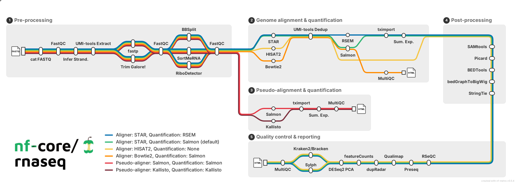
Source: nf-core/rnaseq version 3.26.0.
For this tutorial, we are following the default green path: STAR for alignment and Salmon for quantification. There are multiple valid ways to analyze RNA-seq data, but we will focus on this route.
5 What are FASTQ files?
Sequencing machines produce reads. A read is a short sequence from an RNA molecule. These reads are usually stored in FASTQ files.
FASTQ files often come in pairs:
sample1_R1.fastq.gz
sample1_R2.fastq.gz
For paired-end sequencing:
R1contains the first read from each fragmentR2contains the second read from each fragment.gzmeans the file is compressed
6 What does the pipeline do?
The pipeline takes raw sequencing reads and turns them into quality-control reports, alignments, and expression estimates. These are the major steps shown in the nf-core/rnaseq workflow.
6.1 Pre-processing
These steps clean up and check the raw sequencing reads before alignment or quantification.
- Merge re-sequenced FASTQ files with
cat - Auto-infer strandedness by subsampling reads and pseudoaligning them with
fqandSalmon - Check raw read quality with
FastQC - Extract unique molecular identifiers, if present, with
UMI-tools - Trim adapters and low-quality sequence with
Trim Galore! - Remove genome contaminants with
BBSplit - Remove ribosomal RNA with
SortMeRNA
6.2 Alignment and quantification
After pre-processing, the pipeline can follow different routes. The route depends on whether you want genome alignment, transcript quantification, or pseudoalignment.
The default route used in this tutorial is:
STAR -> SalmonOther available routes include:
STAR -> RSEMHISAT2 -> no quantification- Pseudoalignment and quantification with
SalmonorKallisto
For STAR, the Sentieon implementation can also be chosen if it is available and configured.
6.3 Post-processing
After alignment and quantification, the pipeline organizes and summarizes the mapped reads.
- Sort and index alignments with
SAMtools - Deduplicate reads using UMIs with
UMI-tools, if UMIs are present - Mark duplicate reads with
picard MarkDuplicates - Assemble and quantify transcripts with
StringTie - Create bigWig coverage files with
BEDToolsandbedGraphToBigWig
6.4 Contamination screening
The pipeline can optionally screen selected reads for contamination. By default, this is done on unaligned reads.
Optional tools include:
Kraken2 -> BrackenSylph
6.5 Quality control and reporting
Quality control helps us decide whether the sequencing and analysis worked well enough to trust the results.
The pipeline performs extensive QC with tools such as:
RSeQCQualimapdupRadarPreseqDESeq2MultiQCR
The final report summarizes raw read quality, alignment metrics, gene biotypes, sample similarity, and strand-specificity checks.
7 What do we get at the end?
The main outputs are:
- Quality-control reports
- Alignment or mapping summaries
- Gene or transcript expression estimates
- Pipeline logs and software version information
These outputs help answer questions such as:
- Did the sequencing work well?
- Are any samples low quality or unusual?
- Which genes are expressed in each sample?
- Which samples are ready for downstream analysis?
8 What RNA-seq does not tell us by itself
RNA-seq measures RNA abundance, not every part of biology directly. Gene expression can suggest biological patterns, but interpretation depends on experimental design, replication, annotation quality, and downstream statistics.
Good RNA-seq analysis starts before sequencing. Sample design, metadata, replication, and careful record keeping matter just as much as the computational pipeline.